Classifier Evaluation
I recently wrote an article on our company blog where I explained how we evaluate Machine Learning models at RecordPoint – if you haven’t read it yet, I’d recommend you do so before proceeding.
Since its publishing, I received a number of comments asking me to clarify the concepts presented with concrete examples.
The original article is light on code by design as the audience for the company blog isn’t always that technical. Therefore, in this post I’ll provide a simple example that will hopefully clear things up – in particular why accuracy isn’t enough.
If you’d like to follow along I’ve shared the full source code in a Google Colab Notebook. All you need is a Google account.
A made up skewed dataset
One of the examples I used in the article is a heavily skewed dataset where only 10% of the samples belong to the positive category.
I’ll use the same principle to drive the examples in this post. We’ll start by creating our dataset, X:
sample_size  = 500
num_features = 3
positive_samples = int(0.1 * sample_size) # 10%

# create a matrix of zeroes of shape 500 x 3
X = np.zeros([sample_size, num_features])

# create some noise using random normal distribution
noise = np.random.normal(0,0.5,[sample_size, num_features])
idx = sample_size - positive_samples # 450

# fabricate a relationship for the last 50
# this will improve prediction in our first model
X[idx:, :] = X[idx:, :] + 1

# add noise to the whole dataset
X = X + noise
Next, we create our labels matrix – y – such that 10% are set to the positive category. We also split the dataset into training and testing sets:
# Create predictions
y = np.zeros(sample_size, dtype=np.int64)2

# last 50 samples - 10% - are set to positive
y[marker:] = np.ones(positive_samples, dtype=np.int64)

# Create training and test sets
strat_split = StratifiedShuffleSplit(random_state=42, test_size=0.2) # select 20% as test set

for train_index, test_index in strat_split.split(X, y):
    X_train, X_test = X[train_index], X[test_index]
    y_train, y_test = y[train_index], y[test_index]
Training our model and making predictions
With all setup out of the way we’re ready to train our model. For this example I’ve chosen a DecisionTreeClassifier as we can easily visualize how it predicts classes (see Appendix at the bottom):
clf = DecisionTreeClassifier().fit(X_train, y_train)
print("Accuracy ", clf.score(X_test, y_test))

y_pred = clf.predict(X_test)
print_scores(y_test, y_pred)
plot_confusion_matrix(clf, X_test, y_test, cmap=plt.cm.Blues, display_labels=["Not-HotDog", "HotDog"])
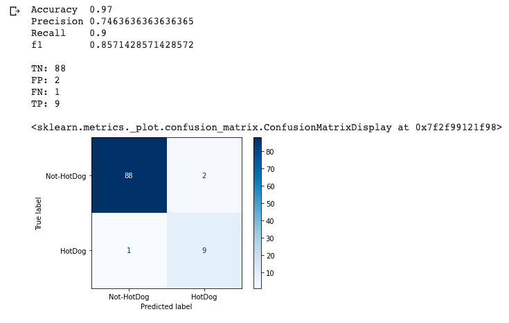
The code above will print the scores we care about: accuracy, precision, recall and f1. In addition it will plot the model’s confusion matrix:

This is an incredibly good model for the random dataset we generated. It achieved 97% accuracy! However, as we know, we shouldn’t stop here. Let’s further evaluate the model using the additional metrics we captured.
We can see that the model’s precision is a bit lower: 75% – that is, it predicted the positive class – hotdog – correctly 75% of the time.
On the flipside its recall is 90% – that is, it correctly identified 90% of all instances labeled “hotdog” in the full dataset.
Lastly the f1 score combines both precision and recall to give us a single measure against which to evaluate the model – 86% in this case and an overall great score.
At this point you’d be asking:
With a 97% accuracy - why did we bother calculating the remaining metrics at all?
Why accuracy isn’t enough
All models are wrong, but some are useful
Let’s create a dumb model that always predicts not-hotdog:
class NotOneClassifier(BaseEstimator, ClassifierMixin):

    def fit(self, X, y):
        self.X_ = X
        self.y_ = y
        return self

    def predict(self, X):
        check_is_fitted(self)
        X = check_array(X)
        return np.zeros(np.ma.size(X,0), dtype=np.int64)
This model literally ignores its input and returns a correctly-sized array of zeros as its predictions.
Your intuition might tell you that this is a terrible model and that it would perform very poorly – but by what measure?
Recall that our dataset is heavily skewed and we have about 10% of positive – hotdog – examples. Let’s see the model performance on that dataset:
dumb_clf = NotOneClassifier().fit(X_train, y_train)
print("Accuracy ", dumb_clf.score(X_test, y_test))

y_pred = dumb_clf.predict(X_test)
print_scores(y_test, y_pred)
plot_confusion_matrix(dumb_clf, X_test, y_test, cmap=plt.cm.Blues, display_labels=["Not-HotDog", "HotDog"])

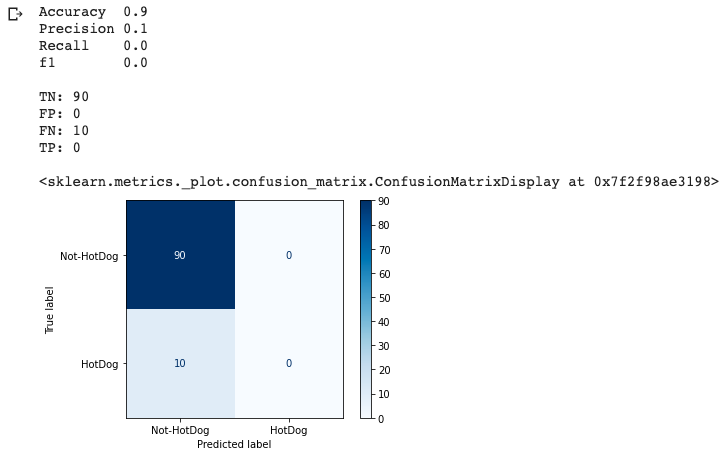
If all we cared about was accuracy we’d look at that 90% and think we have a great model in our hands. This is why precision and recall are so important. Combined they tell a very different story and contribute to a poor score overall.
Of course this is a contrived example but when using real machine learning algorithms, these are the metrics we should be looking at.
Precision and Recall tell us a lot more about our model performance than accuracy alone ever could. They also inform our model parameter-tuning process as we consider the Precision / Recall trade-off for the problem at hand.
Conclusion
Hopefully with a more concrete example the difference between the various metrics became clearer as well as to why they are important.
Don’t forget all source code is available in this Google Colab Notebook.
Appendix
I claimed above that the predictions of a DecisionTreeClassifier are easy to understand – that is, it is an explainable model.
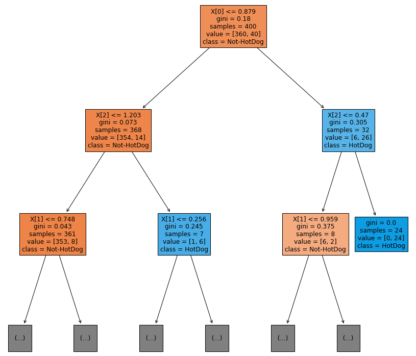
What I mean is that we can plot the decision tree and manually walk through its nodes and branches to understand how the model reached a prediction. For this post’s example, we can plot it using this snippet:
# Just for fun, visualise how the DecisionTree predicts the outcome of the random features

plt.figure(figsize=(15,15))
_ = plot_tree(clf, max_depth=2, filled=True, class_names=["Not-HotDog", "HotDog"])
Which in turn gives us this tree:

The plot is limited to a max depth of 2 so it would fit in this post. However you can see the full plot in the shared Collab notebook.